Intro to Scheduling

OS

CPU Scheduling

Looking at the policies of the Process Dispatcher/Scheduler. What is important when choosing a scheduling algorithm?¹

Assumptions

1. all jobs arrive at the same time
2. once started, each job runs to completion
3. all jobs only use the cpu, no i/o
4. the run time of each job is known

these sound unrealistic (because they are), and we will shed them one by one (some almost immediately)

Metrics

1. Process Metrics
   1. Turnaround Time: time between arrival and completion $$T_{turnaround}=T_{completion}-T_{arrival}$$
   2. Waiting Time: time spent in the ready queue $$T_{waiting}=T_{turnaround}-(\sum T_{cpu}+\sum T_{i/o})$$
   3. Response Time: time before process responds for the first time $$T_{response}=T_{firstrun}-T_{arrival}$$
   4. Fairness²
2. System Metrics
   1. CPU Utilization: %time the cpu is being used
   2. Throughput: number of processes finished in unit time

Gantt Chart

A bar chart that illustrates a project schedule. Different tasks are usually shown on the y-axis, and time intervals on the x-axis

Scheduling Disciplines

First In, First Out (FIFO)

• simple/easy to implement
• efficient to implement, queue operations are $O(1)$

❯ python scheduler.py -l 100,10,10 -p FIFO -c
ARG policy FIFO
ARG jlist 100,10,10
 
Here is the job list, with the run time of each job:
  Job 0 ( length = 100.0 )
  Job 1 ( length = 10.0 )
  Job 2 ( length = 10.0 )
 
Execution trace:
  [ time   0 ] Run job 0 for 100.00 secs ( DONE at 100.00 )
  [ time 100 ] Run job 1 for 10.00 secs ( DONE at 110.00 )
  [ time 110 ] Run job 2 for 10.00 secs ( DONE at 120.00 )
 
Final statistics:
  Job   0 -- Response: 0.00  Turnaround 100.00  Wait 0.00
  Job   1 -- Response: 100.00  Turnaround 110.00  Wait 100.00
  Job   2 -- Response: 110.00  Turnaround 120.00  Wait 110.00
 
  Average -- Response: 70.00  Turnaround 110.00  Wait 70.00

The Convoy Effect

The name comes from a convoy of vehicles. In a moving convoy, when the first car stops, the cars behind it also stop one-by-one. When the first cars move again, the cars at the back are still stopping. The cars in the front can move but all the others have to wait in queue before being able to make progress again

Similarily shorter jobs have to wait in line behind the longer jobs at the front of the queue in FIFO scheduling

Shortest Job First (SJF)

greedy behavious → provably optimal with assumption 1 (all jobs arrive together)

$$T_{waiting}=\frac{0+(t_1)+(t_1+t_2)+(t_1+t_2+t_3)+\dots }{n}$$ $$T_{waiting}=\frac{(n-1)t_1+(n-2)t_2+\cdots +t_{n-1}}{n}$$

For this to be optimal it is clear $t_1\le t_2\le t_3\dots$

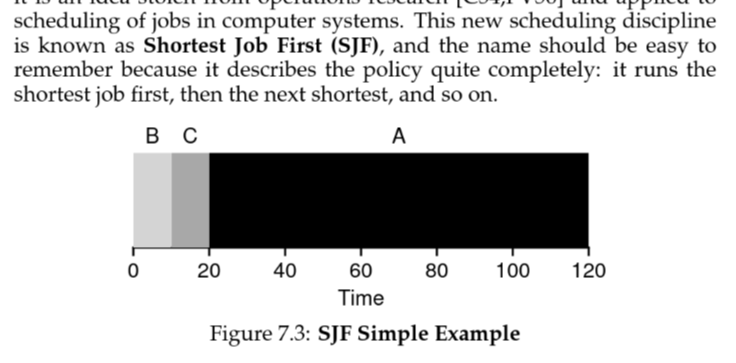
❯ python scheduler.py -l 100,10,10 -p SJF -c
ARG policy SJF
ARG jlist 100,10,10
 
Here is the job list, with the run time of each job:
  Job 0 ( length = 100.0 )
  Job 1 ( length = 10.0 )
  Job 2 ( length = 10.0 )
 
Execution trace:
  [ time   0 ] Run job 1 for 10.00 secs ( DONE at 10.00 )
  [ time  10 ] Run job 2 for 10.00 secs ( DONE at 20.00 )
  [ time  20 ] Run job 0 for 100.00 secs ( DONE at 120.00 )
 
Final statistics:
  Job   1 -- Response: 0.00  Turnaround 10.00  Wait 0.00
  Job   2 -- Response: 10.00  Turnaround 20.00  Wait 10.00
  Job   0 -- Response: 20.00  Turnaround 120.00  Wait 20.00
 
  Average -- Response: 10.00  Turnaround 50.00  Wait 10.00

Non-Preemptiveness

Working under assumption 2, that jobs run to completion, we say we are scheduling non-preemptively.

So if job A (100ms) was to arrive before the other 2 and was scheduled first, we would end up with a situation similar to FIFO (this is bad)

Shortest Time-to-Completion First (PSJF)

Let’s try and resolve the problem with SJF and relax assumptions 1 and 2. Processes now can appear whenever they want, and they no longer run to completition. We call this Preemptive Shortest Job First, and it’s still provably optimal (apparently)

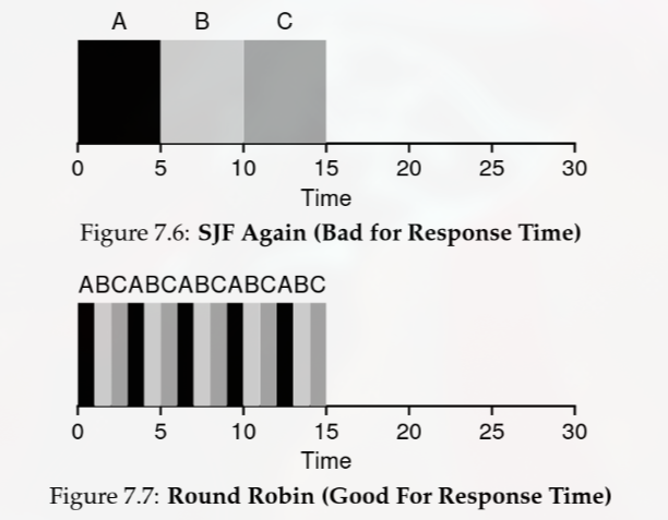
Round Robin

the earlier algs do not consider response time, i.e. the user should get a response from the process they run asap

RR runs a job for a time slice until all jobs are finished

❯ python scheduler.py -l 5,5,5 -p RR -c
ARG policy RR
ARG jlist 5,5,5
 
Here is the job list, with the run time of each job:
  Job 0 ( length = 5.0 )
  Job 1 ( length = 5.0 )
  Job 2 ( length = 5.0 )
 
Execution trace:
  [ time   0 ] Run job   0 for 1.00 secs
  [ time   1 ] Run job   1 for 1.00 secs
  [ time   2 ] Run job   2 for 1.00 secs
  [ time   3 ] Run job   0 for 1.00 secs
  [ time   4 ] Run job   1 for 1.00 secs
  [ time   5 ] Run job   2 for 1.00 secs
  [ time   6 ] Run job   0 for 1.00 secs
  [ time   7 ] Run job   1 for 1.00 secs
  [ time   8 ] Run job   2 for 1.00 secs
  [ time   9 ] Run job   0 for 1.00 secs
  [ time  10 ] Run job   1 for 1.00 secs
  [ time  11 ] Run job   2 for 1.00 secs
  [ time  12 ] Run job   0 for 1.00 secs ( DONE at 13.00 )
  [ time  13 ] Run job   1 for 1.00 secs ( DONE at 14.00 )
  [ time  14 ] Run job   2 for 1.00 secs ( DONE at 15.00 )
 
Final statistics:
  Job   0 -- Response: 0.00  Turnaround 13.00  Wait 8.00
  Job   1 -- Response: 1.00  Turnaround 14.00  Wait 9.00
  Job   2 -- Response: 2.00  Turnaround 15.00  Wait 10.00
 
  Average -- Response: 1.00  Turnaround 14.00  Wait 9.00

compare the final statistics to the same result with SJF

  Average -- Response: 5.00  Turnaround 10.00  Wait 5.00

RR is pretty (very) bad for turnaround time

Choosing the Time Slice

The time quantum $q$ should be larger than the dispatch latency to amortize out context switch overhead. It must also be chosen suitably to minimise turnaround time³

# quantum of 10 -- TAT of 20
❯ python scheduler.py -l 10,10,10 -p RR -c -q 10
  Average -- Response: 10.00  Turnaround 20.00  Wait 10.00
# quantum of 5 -- TAT of 25
❯ python scheduler.py -l 10,10,10 -p RR -c -q 5
  Average -- Response: 5.00  Turnaround 25.00  Wait 15.00
# quantum of 1 -- TAT of 29
❯ python scheduler.py -l 10,10,10 -p RR -c -q 1
  Average -- Response: 1.00  Turnaround 29.00  Wait 19.00

notice the tradeoff between turnaround time and response time (it gets much messier when you start playing with non multiples)

Apparently $q$ is changed adaptively these days based on a lot of stuff. The type of system/process has a lot to with it

• real time systems⁴
• interactive systems
• server systems
• batch systems

Incorporating i/o

relax assumption 3 (no i/o)

still remains basically just PSJF → choose the shortest job at any given time

1. do A
2. A is busy
3. switch to B
4. A is free again
5. switch to A

we’ve dealt with all the assumptions except the last → you never actually know the run time of a process

Estimating Process Runtime

We finally relax assumption 4 (we know the process run time). Since we don’t actually know the runtime, we need to estimate it. To estimate it we look at two factors, the cpu time of the process the last time it ran, and the our previous estimate.⁵

$${\tau }_{n+1}=\alpha t_n+(1-\alpha ){\tau }_n$$

where

• ${\tau }_n$ is our estimate for the $n$th time a process is given the cpu
• $\alpha$ is some constant $0\le \alpha \le 1$
• $t_n$ is the time the process took the last time it had the cpu

we define ${\tau }_0$ as some fair intial value and choose a suitable $\alpha$ for our estimator function

Footnotes

1. Computer Scheduling Methods and their Countermeasures ↩

2. https://en.wikipedia.org/wiki/Fairness_measure lmao ↩

3. i don’t trust this in the slightest but Best Time Quantum RR Alg (they have wikipedia as a reference :sob:) ↩

4. https://www.ibm.com/think/topics/real-time-operating-system ↩

5. analysis of time shared processors i think this discusses the math behind estimating runtime ↩