The Discrete Time Fourier Transform

Signals and Systems

electrical signals systems fourier transforms

---

• Representation of Aperiodic Signals
  • Development of the DT FT
  • Examples of DT FT
  • Convergence Issues with the DT FT
• FT for Periodic Signals
• Properties of the DT FT
  • Periodicity of the DT FT
  • Linearity of the FT
  • Time shifting and Frequency Shifting
  • Conjugation and Conjugate Symmetry
  • Differencing and Accumulation
  • Time Reversal
  • Time Expansion
  • Differentiation in Frequency
  • Parseval’s Relation
• The Convolution Property
• The Multiplication Property
• Duality

---

There are strong parallels between discrete and continuous signals, but there are important differences

• the Fourier Series of a discrete-time periodic signal is a finite series, but the continuous-time representation is infinite
• Similarly there are strong differences in the the Fourier Transforms too.

Representation of Aperiodic Signals: The Discrete-Time Fourier Transform

Derivation

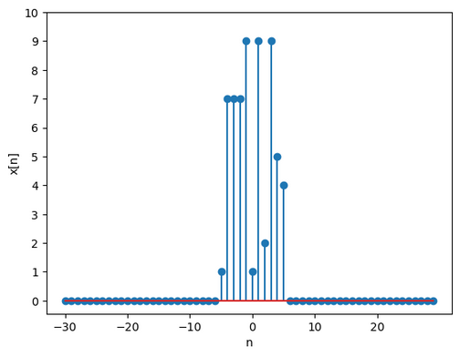
Consider a general sequence $x[n]$ of finite duration as shown below

$x[n]$:

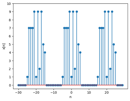
We can construct a periodic sequence $\tilde{x}[n]$ for which $x[n]$ is one period. We can choose the period $N$ as we like, and as $N\to \infty$ we get $\tilde{x}[n]\to x[n]$

$\tilde{x}[n]$:

Now that $\tilde{x}[n]$ is a period function we can take its Fourier Series representation:

$⟨N⟩$ gives you a set over one time period, typically $\{\mathrm{0..}N-1\}$ or $\{\mathrm{1..}N\}$

$$\begin{array}{rl}{a}_k& =\frac{1}{N}\sum _{n=⟨N⟩}\tilde{x}[n]e^{-jk(\frac{2\pi }{N})n}\\ ⟹a_k& =\frac{1}{N}\sum _{n=-\infty }^{\infty }x[n]e^{-jk(\frac{2\pi }{N})n}\end{array}$$

define the Fourier Transform as

$$\begin{array}{rl}X(e^{j\omega })& =\sum _{n=-\infty }^{\infty }x[n]e^{-j\omega }\\ ⟹a_k& =\frac{1}{N}X(e^{jk{\omega }_0})\end{array}$$

where ${\omega }_0=\frac{2\pi }{N}$

$$\begin{array}{rl}\tilde{x}[n]& =\sum _{k=⟨N⟩}{a}_k{e}^{jk{\omega }_{0}n}\\ ⟹\tilde{x}[n]& =\sum _{k=⟨N⟩}\frac{1}{N}X(e^{jk{\omega }_0})e^{jk{\omega }_{0}n}\\ ⟹\tilde{x}[n]& =\sum _{k=⟨N⟩}\frac{{\omega }_0}{2\pi }X(e^{jk{\omega }_0})e^{jk{\omega }_{0}n}\\ & \\ & N\to \infty \\ & \tilde{x}[n]\to x[n]\\ & k{\omega }_0\to \omega \\ ⟹x[n]& =\frac{1}{2\pi }{\int }_{2\pi }X(e^{j\omega })e^{j\omega n}d\omega \end{array}$$

Discrete Time Fourier Transform Representation of Aperiodic Signals:

$$\boxed{\begin{array}{rl}x[n]& =\frac{1}{2\pi }{\int }_{2\pi }X(e^{j\omega })e^{j\omega }d\omega \\ X(e^{j\omega })& =\sum _{n=-\infty }^{\infty }x[n]e^{-j\omega n}\end{array}}$$

• $X(e^{j\omega })$ is periodic unlike the continuous case (with period $2\pi$)
  • this implies that the Fourier Series coefficients $a_k$ are periodic
  • the Fourier Series representation is a finite sum
• the interval of integration is finite in the synthesis equation

signals at frequencies near $\omega =2\pi n$ are considered slow moving or low-frequency signals signals at frequencies near $\omega =(2n+1)\pi$ are considered high-frequency signals

Examples

Consider the function

$$\begin{array}{r}x[n]=a^{n}u[n],|a|<1\end{array}$$ $$\begin{array}{rl}X(e^{j\omega })& =\sum _{n=-\infty }^{\infty }{a}^{n}u[n]e^{-j\omega n}\\ & =\sum _{n=0}^{\infty }{a}^n{e}^{-j\omega n}\\ & =\frac{1}{1-a{e}^{-j\omega }}\end{array}$$

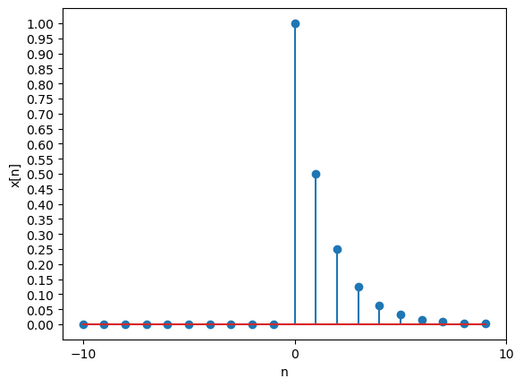
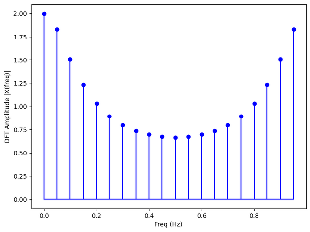
• this Fourier Transform is for $a=0.5$, you can notice that the peaks are concentrated toward $f=0,1$ making this a low-frequency signal.
• Setting $a=-0.5$ makes this a high-frequency graph

Python Function for Graphs

def myFunc(a| n):
    unit = [];
    for sample in n:
        if sample >= 0:
            unit.append(float(a**sample))
        else:
            unit.append(0)
    return unit
UL = 10
LL = -10
n = np.arange(LL, UL, 1)
unit = myFunc(0.5, n)
plt.stem(n, unit)
plt.xlabel('n')
plt.xticks(np.arange(LL, UL + 1, 10))
plt.yticks(np.arange(0, 1.05, 0.05))
plt.ylabel('x[n]')
def DFT(x):
    """
    Function to calculate the 
    discrete Fourier Transform 
    of a 1D real-valued signal x
    """
    N = len(x)
    n = np.arange(N)
    k = n.reshape((N, 1))
    e = np.exp(-2j * np.pi * k * n / N)
    X = np.dot(e, x)    
    return X
sr = 1
X = DFT(unit)
N = len(X)
n = np.arange(N)
T = N/sr
freq = n/T 
plt.figure(figsize = (8, 6))
plt.stem(freq, abs(X), 'b', basefmt="-b")
plt.xlabel('Freq (Hz)')
plt.ylabel('DFT Amplitude |X(freq)|')
plt.show()